Difference between revisions of "Spectral amplitudes"
| (11 intermediate revisions by one other user not shown) | |||
| Line 1: | Line 1: | ||
[[Category:Tutorials]] | [[Category:Tutorials]] | ||
| − | This a short tutorial presenting a step-by-step spectrum procedure. | + | This a short tutorial presenting a step-by-step spectrum procedure using some of the main parameters. |
| + | More details: [[Geopsy: H/V and Spectrum Toolboxes|H/V and Spectrum Toolboxes]] | ||
| Line 23: | Line 24: | ||
* Download [[Media:Strong_peak.tgz|compressed signal file]]. If the file has been already downloaded (as for H/V purposes for example), do not download it again. | * Download [[Media:Strong_peak.tgz|compressed signal file]]. If the file has been already downloaded (as for H/V purposes for example), do not download it again. | ||
* [[Loading and viewing signals|Load and view]] these downloaded signals. | * [[Loading and viewing signals|Load and view]] these downloaded signals. | ||
| − | * Select ''Spectrum'' in menu [[Geopsy: Tools|Tools]] ([[Geopsy: Signal drag&drop#From signal files to the advanced signal processing tools|drag&drop alternative | + | * Select ''Spectrum'' in menu [[Geopsy: Tools|Tools]] ([[Geopsy: Signal drag&drop#From signal files to the advanced signal processing tools|drag&drop alternative way]] to start a tool) |
<br style="clear: both"/> | <br style="clear: both"/> | ||
== Window selection == | == Window selection == | ||
| − | [[Image:SPEC_toolbox_time.png|thumb|right|200px|''General'' sub-tab in ''Time'' tab | + | [[Image:SPEC_toolbox_time.png|thumb|right|200px|[[Geopsy: H/V and Spectum Toolboxes: Time Tab#General sub-tab|''General'' sub-tab]] in [[Geopsy: H/V and Spectum Toolboxes: Time Tab|''Time'' tab]] of toolbox]] |
| − | |||
| − | |||
| − | |||
| − | |||
| − | |||
| − | |||
| − | |||
| − | |||
| − | |||
| − | |||
* Make sure you are in the [[Geopsy: H/V and Spectum Toolboxes: Time Tab|''Time'' Tab]], and that parameters are as in the example window. The ''Anti-triggering on raw signal'' button has been checked. | * Make sure you are in the [[Geopsy: H/V and Spectum Toolboxes: Time Tab|''Time'' Tab]], and that parameters are as in the example window. The ''Anti-triggering on raw signal'' button has been checked. | ||
* To make sure that parameters are set up alright, it is possible to download the [[Media:Spec_Strong_peak.log.tgz|compressed parameter file]] and [[Geopsy: Load Toolbox Parameters|load toolbox parameters]].<br style="clear: both"/> | * To make sure that parameters are set up alright, it is possible to download the [[Media:Spec_Strong_peak.log.tgz|compressed parameter file]] and [[Geopsy: Load Toolbox Parameters|load toolbox parameters]].<br style="clear: both"/> | ||
| − | [[Image:SPEC_toolbox_time_sta.png|thumb|right|200px|''Raw signal'' sub-tab in ''Time'' tab of toolbox with the anti-trigger parameters]] | + | [[Image:SPEC_toolbox_time_sta.png|thumb|right|200px|'[[Geopsy: H/V and Spectum Toolboxes: Time Tab#Raw Signal sub-tab|''Raw signal'' sub-tab]] in [[Geopsy: H/V and Spectum Toolboxes: Time Tab|''Time'' tab]] of toolbox with the anti-trigger parameters]] |
* Click on the [[Geopsy:_H/V_and_Spectum_Toolboxes:_Time_Tab#Raw Signal sub-tab|''Raw signal'']], to check that anti-trigger parameters are as in the example window. As we want the same windowing as in the [[H/V_spectral_ratio|H/V processing]], the ''Common'' button should be checked. | * Click on the [[Geopsy:_H/V_and_Spectum_Toolboxes:_Time_Tab#Raw Signal sub-tab|''Raw signal'']], to check that anti-trigger parameters are as in the example window. As we want the same windowing as in the [[H/V_spectral_ratio|H/V processing]], the ''Common'' button should be checked. | ||
<br style="clear: both"/> | <br style="clear: both"/> | ||
| Line 52: | Line 43: | ||
[[Image:SPEC_toolbox_window_time_postsel.png|thumb|right|200px|Number of selected windows]] | [[Image:SPEC_toolbox_window_time_postsel.png|thumb|right|200px|Number of selected windows]] | ||
| − | * The number of selected windows appears at the bottom right corner of the time tab. The number of windows should be as in the example. | + | * The number of selected windows appears at the bottom right corner of the time tab.<br/> The number of windows should be as in the example. |
<br style="clear: both"/> | <br style="clear: both"/> | ||
[[Image:SPEC_toolbox_result_wind.png|thumb|right|200px|Selected windows]] | [[Image:SPEC_toolbox_result_wind.png|thumb|right|200px|Selected windows]] | ||
| − | * Selected windows should appear as green rectangles on the signal viewer. Here, the windows are synchronous on the three components as we required a common windowing. | + | * Selected windows should appear as green rectangles on the signal viewer. Here, the windows are synchronous on the three components as we required a common windowing in order to compare with the H/V spectral ratio. |
| + | |||
| + | |||
| + | * [[Geopsy: H/V and Spectum Toolboxes: Time Tab#Time windows section |More options]] for selecting windows are available. | ||
<br style="clear: both"/> | <br style="clear: both"/> | ||
| Line 77: | Line 71: | ||
[[Image:HV_toolbox_no_window_selected.png|thumb|right|200px|No selected windows pop-up window]] | [[Image:HV_toolbox_no_window_selected.png|thumb|right|200px|No selected windows pop-up window]] | ||
| − | * In case no window selection has been performed, a | + | * In case no window selection has been performed, a pop-up window appears. |
Simply click on the ''Yes'' button and processing will follow its way. | Simply click on the ''Yes'' button and processing will follow its way. | ||
| Line 90: | Line 84: | ||
==== Spectrum curves ==== | ==== Spectrum curves ==== | ||
[[Image:SPEC_toolbox_SPEC_1.png|thumb|right|200px|Timing tab in toolbox]] | [[Image:SPEC_toolbox_SPEC_1.png|thumb|right|200px|Timing tab in toolbox]] | ||
| − | * As the spectrum has been computed on each component, the | + | * As the spectrum has been computed on each component, the figure is divided in three different graphs. |
* In each graph, the black curve represents the spectrum averaged curve over all colored individual spectrum curves The two dashed lines represent spectrum standard deviation. | * In each graph, the black curve represents the spectrum averaged curve over all colored individual spectrum curves The two dashed lines represent spectrum standard deviation. | ||
| − | |||
<br style="clear: both"/> | <br style="clear: both"/> | ||
[[Image:SPEC_toolbox_SPEC_pick_value.png|thumb|right|200px|Peak frequency and standard deviation values]] | [[Image:SPEC_toolbox_SPEC_pick_value.png|thumb|right|200px|Peak frequency and standard deviation values]] | ||
| Line 105: | Line 98: | ||
== Changing spectrum graphics appearance == | == Changing spectrum graphics appearance == | ||
[[Image:SPEC_toolbox_makeup.png|thumb|right|200px|''Output'' tab showing an example to use a make-up ]] | [[Image:SPEC_toolbox_makeup.png|thumb|right|200px|''Output'' tab showing an example to use a make-up ]] | ||
| − | * It is possible to change the appearance of the spectrum graphics at the user's will using a make-up. | + | * It is possible to change the appearance of the spectrum graphics at the user's will, using a make-up. |
* As an example, first download the [[Media:SPEC_makeup.mkup.tgz|compressed make up file]]. | * As an example, first download the [[Media:SPEC_makeup.mkup.tgz|compressed make up file]]. | ||
** Then go to the ''Output'' tab; | ** Then go to the ''Output'' tab; | ||
Latest revision as of 12:08, 15 April 2010
This a short tutorial presenting a step-by-step spectrum procedure using some of the main parameters.
More details: H/V and Spectrum Toolboxes
Contents
Introduction
This tool is used to obtain Fourier amplitude spectra from any type of vibration signals (ambient vibrations, earthquake…). The example used for explanations is an ambient vibration recording on soil.
As for the other tools, the data can be processed:
- from a graphic viewer, to verify the windowing and to display the results;
- from a table. In this case, Geopsy will display only the resulting curves.
A global description of the Spectrum Toolbox is available for more details.
Getting ready
- Download compressed signal file. If the file has been already downloaded (as for H/V purposes for example), do not download it again.
- Load and view these downloaded signals.
- Select Spectrum in menu Tools (drag&drop alternative way to start a tool)
Window selection
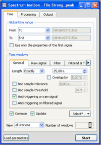
- Make sure you are in the Time Tab, and that parameters are as in the example window. The Anti-triggering on raw signal button has been checked.
- To make sure that parameters are set up alright, it is possible to download the compressed parameter file and load toolbox parameters.
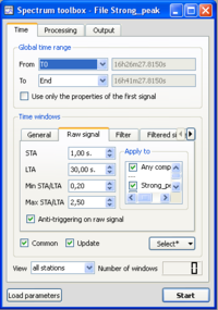
- Click on the Raw signal, to check that anti-trigger parameters are as in the example window. As we want the same windowing as in the H/V processing, the Common button should be checked.
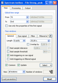
- Click on the Select button and select Auto into the pop-up menu.
- The number of selected windows appears at the bottom right corner of the time tab.
The number of windows should be as in the example.
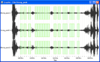
- Selected windows should appear as green rectangles on the signal viewer. Here, the windows are synchronous on the three components as we required a common windowing in order to compare with the H/V spectral ratio.
- More options for selecting windows are available.
Processing parameters
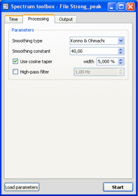
- Click on the Processing tab, and make sure that parameters are as in the example window.
Output parameters
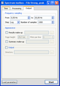
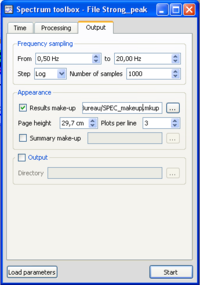
- Make sure you are in the Output tab, and that parameters are as in the example window.
Data processing
- In case no window selection has been performed, a pop-up window appears.
Simply click on the Yes button and processing will follow its way.
Results
Signal display
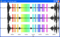
- Selected windows are colored, matching colours in the spectrum graphics, i.e. colour of individual spectrum curves have the same colour as the signal windows.
Spectrum curves
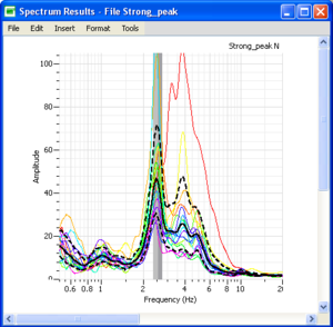
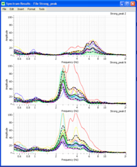
- As the spectrum has been computed on each component, the figure is divided in three different graphs.
- In each graph, the black curve represents the spectrum averaged curve over all colored individual spectrum curves The two dashed lines represent spectrum standard deviation.
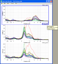
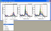
- Use the cursor to get values on the spectrum curves. The exact value of the spectrum peak frequency and its standard deviation may be obtained by sliding the cursor onto the spectrum curve title (Strong_peak Z, Strong_peak N, Strong_peak E) in the upper right corner above the graphics.
Synthetic graph
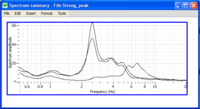
- For the spectrum computation, a synthetic graph displays the averaged spectrum curves coming from each waveform.
Changing spectrum graphics appearance
- It is possible to change the appearance of the spectrum graphics at the user's will, using a make-up.
- As an example, first download the compressed make up file.
- Then go to the Output tab;
- In Appearence section, chek the Results make-up button;
- Browes (click on the following cursor
 ) in the hard drive to find the "SPEC_makeup.mkup" file and select it.
 - The line below, in the Plots per line area, enter 3 (giving 3 graphs per line)

- Click again on the start button to apply the appearance.
- The appearance of the spectrum graphics is now at the user's taste.
Saving results
There are two solutions to save the results graphically. The first one allows saving each individual graph in independant files and the second allows saving all the graphics onto the spectrum results graphic window in a single file.
- Saving the graphs in individual files
- The spectrum graphics may be saved in various image formats.
- Right click in the left hand margin of the spectrum graphic.
- In the pop-up menu, choose Export image. Then choose a destination.
- Saving all the graphs in a single file
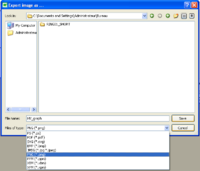
- Select Export image in the File sub-menu.
- Choose a destination folder, image format, and file name.
