Difference between revisions of "Dispersion curve inversion"
| Line 18: | Line 18: | ||
Load a dispersion curve and fix its frequency sampling: | Load a dispersion curve and fix its frequency sampling: | ||
| − | * Load | + | * Load a dispersion curve from a text file (e.g. [[Media:Test_Rayeigh_2modes.disp|Test_Rayeigh_2modes.disp]]). It is a theoretical curve computed using tutorial [[Computing a theoretical dispersion curve]]. |
| + | [[Image:Dinverdc_loaddc.png|thumb|center|200px|Loading a dispersion curve]] | ||
* Select the fundamental curve | * Select the fundamental curve | ||
::Use ''curve data scroll bar'' and ''visible button'' to identify it. | ::Use ''curve data scroll bar'' and ''visible button'' to identify it. | ||
Revision as of 10:58, 23 February 2010
This tutorial shows how to invert a dispersion curve measured for surface waves. It is based on dinverdc module used inside dinver framework.
Contents
Getting ready
Start Dinver with Surface Wave Inversion module.
At first glance, the interface might look a little bit messy. If it is the first time you start dinver, you'd better close all windows until having an empty workspace. The various tools will be displayed one by one and explained in this tutorial, in a logical order.
Importing the dispersion curve to fit
- Activate the Target panel in menu Tools.
- Select the Dispersion option. Leave the Misfit weigth and the Min. misfit to their default values, 1 and 0, respectively.
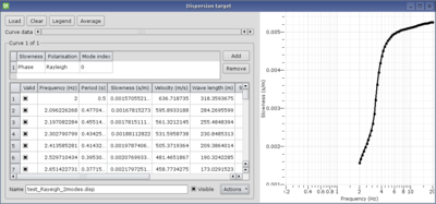
- Click on Set to load the dispersion curve, the Dispersion curve target is displayed.
Load a dispersion curve and fix its frequency sampling:
- Load a dispersion curve from a text file (e.g. Test_Rayeigh_2modes.disp). It is a theoretical curve computed using tutorial Computing a theoretical dispersion curve.
- Select the fundamental curve
- Use curve data scroll bar and visible button to identify it.
- This is the curve defined over the complete frequency range and with higher slowness).
- Re-sample it from 2 to 20 Hz on log scale with 50 samples (menu Actions/Resample).
- Cut it from 2 to 20 Hz (menu Actions/Cut).
- Select the first higher mode curve
- Use curve data scroll bar and visible button to identify it.
- This curve is not defined over the complete frequency range and it has a lower slowness).
- Remove it (menu Actions/Remove).
Achieving a good frequency sampling is an art, for a better understanding see Curve sampling.
At this step, the Dispersion curve target should contain only one curve, the fundamental mode. Make sure the mode table contains only one item like this:
Defining the parameter space
Defining the parameter is the key point of the inversion. At this step you have to figure out what information you already know about the ground structure and information you would like to extract. More details on how to achieve a good parameterization.
- Activate the Parameter panel in menu Tools.
- Add two layers for Vp profile by clicking on Add button in Compressional velocity profile.
- Add one layer for Nu profile by clicking on Add button in Poisson's ratio profile.
- Add two layers for Vs profile by clicking on Add button in Shear velocity profile.
- Add one layer for Rho profile by clicking on Add button in Density profile.
- Link Vp interface to Vs interface by selecting Vs0 in Linked to combo box.
Currently the parameterization describes a ground structure with one layer over a half-space with uniform Vp and Vs in the top and bottom layer. The default range for values is relatively large. Vp contrast is forced to be at the same depth of Vs contrast, and only one parameter for depth is kept. Poisson's ratio is not a parameter but a condition imposed to Vp and Vs values: computed Poisson's ratios must be between 0.2 and 0.5. The panel should look like this one:
Running the inversion
Before going any further, it is wise to save the current environment, i.e. the target and parameter space definitions into a .dinver file. Select maneu File/Save as .... Target and parameterization defined here above are available with file Dinverdc_tutorial-1.dinver.


