Max2curve

Visualization of analysis statistics

max2curve is a graphical user interface for visualization analysis results of various processing options in geopsy. max2curve reads, filters and determines histograms from .max files.

You may call max2curve on the command line directly with the output file (.max file) produced from your f-k processing.

$> max2curve your_output_file.max

Startup of max2curve for selecting histogram parameters - FK case

Startup of max2curve for selecting histogram prameters - SPAC case

Startup of max2curve for selecting histogram prameters - HVTFA case

Certainly you may also open max2curve directly. Then you will need to locate your .max file in the directory tree and select it with the automatically opened file browser.

max2curve then reads the contents of the .max output file and computes a probability density function (pdf) for slowness values (in case of f-k result files) or autocorrelation values (in case of MSPAC output files) for each individual frequency band of processing.

In order to be able to produce the pdf from re-normalization of a binned histogram, max2curve needs to know about:

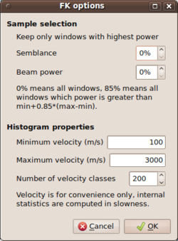
• the slowness limits and the number of bins to use for the f-k output files.
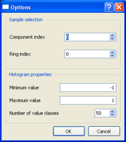
• the ring and component index, limits for the autocorrelation values (-1,1 is a good choice) and number of bins to use for the spac output files.
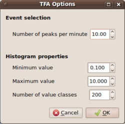
• the limits of the ellipticity values (0.1,10 is a good choice) and number of bins to use for the H/V tfa output files.

An example for the usage of max2curve in either case are given in the FK tutorial, the MSPAC tutorial, and the H/V tfa tutorial, respectively.

Further, for each of the three output file types, it is possible to make a pre-selection or some filtering according to method specific criteria.

• For the f-k type output results, it is possible to filter the .max file(s) according to two extra criteria. Using the two entries under Sample selection, i.e. specify percentage values for Semblance and Beam power, it is possible to filter individual time window results falling below thresholds for the semblance coefficients and beam power values. Although semblance is a normalized quantity, we choose to develop a relative threshold scheme for filtering results for both semblance and beam power values. The percentage values should be understood as follows: for all entries in the .max output file, the minimum and maximum values for the semblance coefficient and the beam power values are used as lower (0%) and upper (100%) limits. Any given percentage value will compute the threshold as absolute value in between these two limits by linear interpolation. Note that the conditions are combined in the sense of a logical and. Only time window that surpass the threshold for both values (semblance and beam power) will be kept and passed to the histogram computation. Any other analysis window result will be skipped and is not taken into account for the computation of the frequency dependent histogram.
• For the MSPAC type output results, the results will be filtered according to some ring and component index. The output files contain the autocorrelation values for each ring and component for each analysed time window. For computing a histogram it makes only sense to select the results for one ring and component. Component indices from 0 to 2 (Vertical=0, Radial=1, Transverse=2) are only needed for 3C-MSPAC computation.
• For the HVTFA type output files, the criterion for selection is based on a maximum number of events per minute to be kept for the final analysis. NEEDS MORE DESCRIPTION (Mirjam??)

TO BE CONTINUED

Grid statistics window

Grid statistics window of max2curve

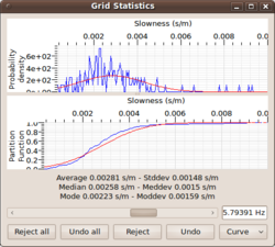
The Grid statistics window allows the user of max2curve to visualize the histograms for each frequency. To scan over different frequency bands, one can use the slider bar to scan from the lowest to the highest frequency band. For some selected center frequency, one obtains the re-normalized histogram ( = pdf) of all slowness estimates in the upper panel. The sample mean $\mu (f_{c})$ and sample standard deviation $\sigma (f_{c})$ calculated from the histogram are used to display the corresponding normal distribution $N(\mu (f_{c}),\sigma (f_{c}))$) as overlaying red curve.

The lower panel shows the same information, but displayed as cumulative histogram or probability function instead of histogram and pdf. The display has been introduced because it is often easier to recognize the proximity of a distribution to the normal distribution in the cumulative view.

Besides the visualization, the grid statistics window can be further used to modify/edit/clean the histograms on grounds of expert knowledge about the way aliasing phenomena are wrapped into the histogram picture. Details about the editing capabilities and final dispersion curve determination may be found in this page.