Ambient vibration array

F-K Toolbox (conventional f-k)

Opening f-k toolbox - overview

Signal viewer for one group of simultaneously recorded waveforms ready for array processing

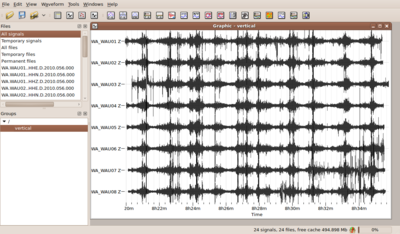
If you have followed all steps above you should have now a set of simultaneously recorded waveforms building a group and containing coordinates for each waveform. You can view this group of waveforms in the data viewer and should get a picture like the one shown to the right.

Now you can open the conventional frequency wavenumber toolbox by pushing the plugin icon .

The f-k toolbox should open and is now attached to the signal viewer. No other toolbox will now open with the signals you have loaded to the signal viewer. In order to process the same data set by another tool, you have to open them in a different signal viewer window. Note also, that once you close either the f-k toolbox window or the signal viewer, there is no way to undo this action - you will have to start again by opening a new signal viewer and attaching the f-k toolbox to it. Alternatively you can drag your group directly into the f-k toolbox icon. Geopsy will automatically open a new exclusively attached signal viewer for you.

Conventional f-k toolbox

Let's now have a close look to the individual parameters to be set in the f-k toolbox. There are four main groups of parameters to be considered.

• Pre-processing parameters for excluding data from processing.
• Processing parameters for selecting time windows on the remaining data.
• Processing parameters for selecting narrow frequency bands for processing
• Parameters related to the output of results from f-k processing.

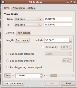
These parameters are laid out in different parts of the f-k toolbox widget. Note, that the toolbox has three main tabs: Time, Processing and Status.

The pre-processing parameters for excluding data from processing follow the same argumentation as the data selection for other toolboxes like H/V processing and can be found in the Time tab.

E.g. one can apply the so-called anti-trigger approach for removing transient signals from the continuous recordings (i.e. excluding those time chunks from processing). The anti-trigger approach can be applied to raw or filtered data. For the detailed settings please look into the description of anti-trigger. Another, second, approach for excluding data from processing is provided via the bad sample approach. For details in setting parameters with the bad sample approach check this page.

Parameter settings

Parameters for time window settings

Time limits layout group

There are two distinct inputs in the f-k toolbox for selecting time windows for processing. First, it is necessary to specify start and end times of the overall data window for processing by selecting entries From and To in the Time limits part of the Time tab of the fk-toolbox.

There are three options each for the drop boxes From and To. For the From entry you can select among .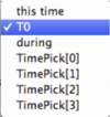

• this time (entries in form xx h xx m xx.xxx s)
• T0 (selects earliest common start time of all traces in group)
• during (selects time duration before end of the signals - either specified with End or this time as explained below)

For the To entry there are the options :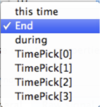

• this time (entries in form xx h xx m xx.xxx s)
• End (selects latest common end time of all traces in group)
• during (selects time duration from start time as given above - either specified by this time or T0)

Note: a selection of time limits as From: during && To: during is NOT valid.

General tab

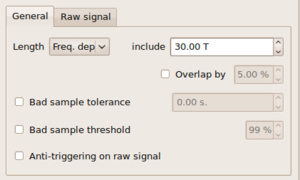
After selecting the overall data window for processing you finally have to specify the window length for each single analysis window to be processed. You can find this Length parameter in the General tab inside the Time tab. There are again three options provided in a drop box .

• Exactly (takes exactly the time window length as provided in the corresponding editable box - unit is in seconds).
• At least (takes at least the time window length as given in the editable box, if possible it takes more - unit is in seconds).
• Freq. dep. (read: frequency dependent. Scales window length to the center frequency of each frequency band to be processed. The number given in the editable box corresponds to a window length in number of cycles for each frequency band. T is the center period of the band).

Note: the most common setting for the Length parameter is Freq. dep. with values between 20.00 to 50.00 meaning that 20 to 50 cycles of the central siganl period per frequency bands are used as window length. Example: for a frequency band with center frequency 2.5 Hz, the central period is 1/2.5 = 0.4 s. Therefore, with a frequency dependent Length setting of 30.00 T, the window length will be chosen as 12.00 s.

Parameters for frequency band selection

Processing tab of f-k toolbox

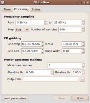
The selection of the frequency bands to be processed is driven by parameter inputs inside the Processing tab of the f-k toolbox. In the Frequency sampling layout group you can specify the minimum and the maximum (central) frequencies for processing. Between these two limits, the frequency axis will then be sampled according to the settings in the next line .

There are two options to be specified, namely Step and Number of Samples. For the Step parameter, there are two options to be selected from a drop box: Log or Linear. You might have guessed the meaning right away. When choosing Linear then the frequency axis is sampled linearly between the given limits and exactly Number of Samples will be distributed along the axis. Choosing Log accordingly samples the frequency axis logarithmically, i.e. frequency bands are close spaced at lower frequencies.

Note: the sampled frequencies are taken as center frequencies in the processing scheme. Therefore, it is necessary to specify additionally a bandwidth so that the processing can be performed in a finite but narrow frequency band. The bandwidth parameter is chosen as relative half-bandwidth in the FK-gridding layout group in the processing tab .

The frequency limits for each frequency band are computed as $[(1-bw)\cdot f_{c},(1+bw)\cdot f_{c}]$ where $f_{c}$ is the central frequency and $bw$ is the bandwidth parameter.

Example: a setting of 0.10 for the bandwidth, a Linear spacing of 10 samples along the frequency axis from 1 Hz to 10 Hz will create the following frequency bands:

Frequency band creation using Step: Linear, Bandwidth: 0.10, From: 1 Hz, to: 10 Hz

Freq. band index	Lower frequency limit	Center frequency	Upper frequency limit
1	0.9 Hz	1.0 Hz	1.1 Hz
2	1.8 Hz	2.0 Hz	2.2 Hz
3	2.7 Hz	3.0 Hz	3.3 Hz
4	3.6 Hz	4.0 Hz	4.4 Hz
5	4.5 Hz	5.0 Hz	5.5 Hz
6	5.4 Hz	6.0 Hz	6.6 Hz
7	6.3 Hz	7.0 Hz	7.7 Hz
8	7.2 Hz	8.0 Hz	8.8 Hz
9	8.1 Hz	9.0 Hz	9.9 Hz
10	9.0 Hz	10.0 Hz	11.0 Hz

Parameters influencing the sampling of the wavenumber space

The basic idea of f-k processing consists of delaying the observed recordings at different stations according to a particular horizontal wavenumber vector ${\vec {k}}=(k_{x},k_{y})^{T}$ and computing the coherence and/or beam power of the shifted stacked output of all array stations.

• Beampower:

$BP(\omega ,{\vec {k}})=\sum _{\omega =\omega _{l}}^{\omega =\omega _{h}}\left[\sum _{i=1}^{i=N}X_{i}(\omega )\exp(j{\vec {k}}{\vec {r}}_{i})\right]^{2}$

• Semblance:

$Semb(\omega ,{\vec {k}})={\frac {\sum _{\omega =\omega _{l}}^{\omega =\omega _{h}}\left[\sum _{i=1}^{i=N}X_{i}(\omega )\exp(j{\vec {k}}{\vec {r}}_{i})\right]^{2}}{N\sum _{\omega =\omega _{l}}^{\omega =\omega _{h}}\sum _{i=1}^{i=N}\left[X_{i}(\omega )\exp(j{\vec {k}}{\vec {r}}_{i})\right]^{2}}}$

$X_{i}(\omega )$ is the observed record at station $i$ at frequency $\omega$. The station coordinates in the array plane (usually earth's surface) are given by ${\vec {r}}_{i}$. By testing many wavenumber vectors in the wavenumber plane one tries to find those wavenumbers which maximize the array output. The wavenumber found corresponds to a plane wave along the surface crossing the seismometer array. So, the problem at hand is a general optimization problem trying to find the maximum of a function of two parameters (here $(k_{x},k_{y})^{T}$). In order to optimize the grid search approach, the f-k toolbox relies on the following sampling strategy.

Graphical display of f-k results using max2curve

max2curve

High resolution frequency wavenumber Toolbox (Capon's method)

The high resolution frequency wavenumber (hrfk) algorithm follows the ideas of Capon (1969)

. The corresponding toolbox that can be called using the following plugin icon can be used straightforward in nearly the same way as the conventional f-k toolbox.

There is just one more (optional!) parameter that can be set. The calcuation for the hrfk algorithm involves the inversion of the cross spectral matrix estimate from the data. In order to guarantee a numerically stable solution for the Matrix inversion, a regularization parameter (damping constant) can be provided to load the diagonal of the cross spectral matrix before inversion.

Note: by doing so (using a damping constant), you will smooth out your wavenumber power spectra and eventually not obtain much better results compared to the conventional beamforming approach.

Modified Spatial Autocorrelation (MSPAC) Toolbox

The Modified Spatial Autocorrelation (MSPAC) was introduced by Bettig et al. (2001) after pioneer paper of Aki (1957). This method allows computing spatial autocorrelation coefficients for any arbitary array layouts.

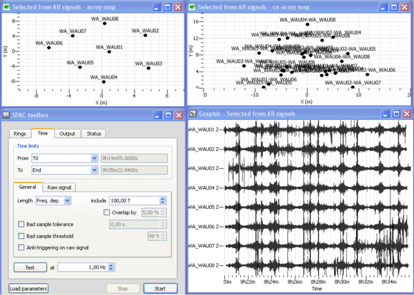
After viewing the group of waveforms in the data viewer, open the MSPAC toolbox by pushing the following plugin icon . Alternatively you can drag your group directly into the SPAC toolbox icon. The SPAC toolbox should now be attached to the signal viewer. Four windows should then opened as displayed in the figure on the right: (1) a signal time viewer, (2) a map displaying array station locations, (3) a map displaying co-array stations location and (4) the SPAC processing toolbox. This processing toolbox is composed of four sub-menus: "Rings" sub-menu is used to design rings from the co-array; "Time" is used to define begin and end time to be processed, time window length, anti-triggering options as described in section XXX; "Output" menu is used to set up the output frequency band together with the sampling scale type (linear, log) and number of frequencies, the output filename; "Status" menu provides information about computing status. All these sub-menus are described hereafter.

Steps involved in the design of the rings.

Defining rings

In "rings" sub-menu:

• Push on button to add a ring
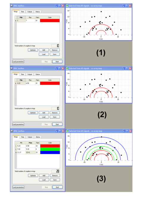
• Specify the inner and outer circles radii of the ring (see step (1) in the figure on the left)
• Press on buttom to adjust the inner and outer circles radii in order to fit at best sensors location (see step (2) in the figure on the left). This ring is composed of 10 pairs of sensors as specified in the "Pairs" column.
• Define the next rings (see step (3) in the figure on the left). Note that you can associate a specific color to each ring.
• Note that you add or remove specific ring by pushing on the or buttons
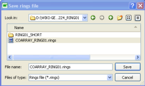
• Once done, click on to save your rings design.

• The rings design can next be loaded by pushing on the button
• the rings design are saved in ascii format with the following format: inner circle radius (in meters), outer circle radius (in meters), RGB color code associated to the ring

Rings definition format

Defining time limits

In "Time" sub-menu:

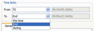
• Select the time limits to be processed. You can either use the begin To and end time End of the time series, either specify the begin and end time This Time or specify the time duration Duration

• Specify the window length that will be used for processing. You can either choose a window length that is inversely proportionnal to the frequency of interest Freq. Dep., a fixed time window length Exactly or a variable length limited by a minimum and a maximumm At Least.
• By pushing on , you can also load the .log file containing all the input parameters saved from a previous computation (see Editing spatial autocorrelation curves for complementary information).

Defining the outputs and starting the computation

In "Output" sub-menu:

• Choose the frequency band used for the computation
• Specify the number of frequencies and the sampling scale (constant on a linear or logarithmic scale).

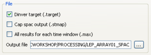
• Click on Dinver target to save your results in a .target file. Set the output filename.
• Then, click on to start the computation. Status of the computation can be checked in the "Status" sub-menu as displayed below.

Editing spatial autocorrelation curves

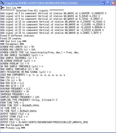
The spatial autocorrelation coefficients and the parameters used for the computation are saved in a .target binary file and a .log ascii file, respectively. The .log file is saved in the same folder as the .target file. The figure on the right displays the content of the .log file.

Graphical display of f-k results using spac2disp

spac2disp

Further readings

• Frequency Wavenumber
• High Resolution Frequency Wavenumber

References

- ↑ Capon, 1969. xxx ,IEEE Proceedings, , , .
- ↑ Bettig B., P.-Y. Bard, F. Scherbaum, J. Riepl, F. Cotton, C. Cornou, D. Hatzfeld, 2001. Analysis of dense array measurements using the modified spatial auto-correlation method (SPAC). Application to Grenoble area., Boletin de Geofisica Teoria e Applicata, 42, 3-4, 281-304.
- ↑ Aki, K., 1957. Space and Time Spectra of Stationary Stochastic Waves, with Special Reference to Microtremors, Bull. Earthq. Res. Inst. Tokyo, 35, 415-457.
![{\displaystyle [(1-bw)\cdot f_{c},(1+bw)\cdot f_{c}]}](https://wikimedia.org/api/rest_v1/media/math/render/svg/0fe99391fce970338a12a0d88a61cb43a1e40295)
![{\displaystyle BP(\omega ,{\vec {k}})=\sum _{\omega =\omega _{l}}^{\omega =\omega _{h}}\left[\sum _{i=1}^{i=N}X_{i}(\omega )\exp(j{\vec {k}}{\vec {r}}_{i})\right]^{2}}](https://wikimedia.org/api/rest_v1/media/math/render/svg/8636e618e5e7ae5f97b3c9cbc758b2359cf76dc0)
![{\displaystyle Semb(\omega ,{\vec {k}})={\frac {\sum _{\omega =\omega _{l}}^{\omega =\omega _{h}}\left[\sum _{i=1}^{i=N}X_{i}(\omega )\exp(j{\vec {k}}{\vec {r}}_{i})\right]^{2}}{N\sum _{\omega =\omega _{l}}^{\omega =\omega _{h}}\sum _{i=1}^{i=N}\left[X_{i}(\omega )\exp(j{\vec {k}}{\vec {r}}_{i})\right]^{2}}}}](https://wikimedia.org/api/rest_v1/media/math/render/svg/8cd1438756296c3a82fa4684147d75be524eb560)