Gplivemodel

gplivemodel computes dispersion curves, autocorrelation curves, ellipticity curves or SH tranfert functions from a layered model. Compared to command line tools like gpdc, gpspac, gpell and gpsh, ground models can be interactively modified in a graphical user interface.

Important: this is not an inversion tool. Manually inverting a dispersion curve with this tool leads to an extremely poor and biased estimation of the global solution of the inversion problem. dinver is a much more appropriate inversion tool.

Description

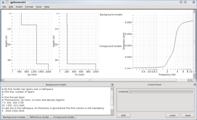
Gplivemodel graphic interface with a background model.

gplivemodel graphical interface is structured in 3 panes:

• Plots of Vp and Vs profiles, and the computed curve (top of figure)
• Model definition (bottom left of figure)
  • Background models
  • Reference model
  • Foreground model
• Control panel (bottom right of figure)

Background models and Reference model are free text editors containing layered model descriptions. Model format is the same as for gpdc, gpspac, gpell or gpsh. Control panel has a collection of sliders to control the transformation of Reference models into Foreground models. A right-click on a slider lets the user editing the effects.

Above plots (included in a graphic sheet) are continuously updated after any modification of Background models, Reference models editors or Control panel. Any number of model descriptions can be entered there. By default, axis limits are also changed. To preserve their current state, menu Format has option Automatic limits to be checked or not.

Attributes (color, symbols,...) of velocity profiles and computed curves can be set be editing the legends located on the left of the curve plot.

Tutorials

• Dispersion curve
• Autocorrelation curve
• Ellipticity curve
• SH transfer function

Slider definition

A slider to control the first layer thickness

A slider has a name displayed on the left. This name can be edited in the same dialog box as the slider action. A slider has a value (called p for parameter). This variable is 0 when the cursor is on the left end and 1 when it is on the right end. It can take any of the 101 discrete values between 0 and 1. Reference models are described by 4 (or 6 for SH only) vectors:

• h for thicknesses (m)
• vp for compressional wave velocities (Vp, m/s)
• vs for shear wave velocities (Vs. m/s)
• rho for densities (kg/m3)
• Qp for compressional wave attenuation factors
• Qs for shear wave attenuation factors

n is a constant containing the number of layers.

Any value of these vectors can be changed by any number of formulas.

h[0]=5+p*95;

It defines a slider that modifies the thickness of the first layer from 5 to 95 m.

r=h[0]*v[0];
v[0]=100+p*300;
h[0]=r/v[0];

It defines a slider that modifies the velocity keeping a constant travel time in the first layer