Geopsy: H/V and Spectrum Toolboxes: Output Tab

Output tab where the user can fix the parameters to display and save the results

Through this tab, the user is able to fix the parameters to display and save the results.

This tab is divided in three sections:

• Frequency sampling section: where the user can fix the parameters on frequency limits and more.

• Appearance section: where the user can fix automatic output graphics appearance parameters.

• Output section: where the user can fix where to save data.

Frequency sampling section

Frequency sampling section where the user can fix the parameters on frequency limits and more

In this section describes how to fix the upper and lower limits (in the frequency domain) for computing. This part is strongly linked to the properties of the Fourier transform.

• The lower limit should be fixed in two different ways :
  • The first possibility is to fix the lower frequency limit equal to the natural frequency of the sensor.
  • From SESAME guidelines , the other possibility is to define the lower frequency limit from the window length, taking into account the following formula ${\frac {10}{w_{l}}}>f_{seismometer}$. Where ${w_{l}}$ is the window length and $f_{seismometer}$ the natural frequency of the sensor.
    Example 1, if the windows have been fixed to exactly 25 seconds, the lower frequency limit is 0.4 Hz.
    Example 2, if the natural frequency of the sensor is 0.2 Hz, the lower frequency limit is 0.2 Hz (giving a maximum window length of 50 seconds).
    Example 3, if the natural frequency of the sensor is 0.2 Hz and the window length has been fixed to 25 seconds, the higher frequency should be used. In this case: 0.4 seconds
    
    Of course, it is always possible to pass over this limitation by computing and viewing at lower frequency, but in this case, the user shoud keep in mind that the data below the "theorical" limit are useless. Moreover, in the graphics of H/V or Spectrum a red dashed area will appear in the frequencies below the ${\frac {10}{w_{l}}}$ frequency as a reminder.

• The maximum upper limit is fixed by the Nyquist frequency, which corresponds to the half of the digitization frequency sampling. If the signal has a 100 Hz sampling frequency, the Nyquist frequency will be 50 Hz.
  Above Nyquist frequency, due to the Fourier transform in itself, no data are available. So there is no need to go above the Nyquist frequency.
  Below Nyquist frequency, there is no lower limit to the upper limit, except the lower limit frequency.
  In general, the upper limit is fixed in-between a 10-50 Hz frequency range.
• Two options have to be fixed
  • Step: option to define how the sampling of the Fourier transform (along the given limits, lower limit and upper limit) will be distributed. A drop box proposes two possibilities for the sampling:
    • Lin, for linear sampling. In this case, the samples are linearely distributed in the frequency domain.
    • Log, for logarithmic sampling. In this case, the samples are logarithmically distributed in the frequency domain.
  • Number of Samples. This spin box allows the user to define the number of samples needed to process the Fourier transform.

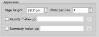
Appearance section

It is possible to set-up automatic graphics output appearance parameters

Output section

Unactivated Output section. The user is unable to save the data.

Activated Output section displaying where (on the hard drive) the user is saving the data.

Browser allowing the user to choose the folder to save the results. In this browser, the user can also create folder.

The user can define where in his hard drive the results will be saved. To do this, first it is necessary to check the Output box and then, the user has to click on the following cursor to open a brower to navigate in the hard drive to find the folder where the result files should be saved.

Following the use, H/V or Spectrum, the output files are different:

• for H/V processing. For each three components group (N-E-Z) the results are saved in two different files: name.log and name.hv, where 'name' stands for the station name:
  • the .log files in which the H/V parameters are stored (Example). In this file the windowing is also saved.
  • the .hv files in which H/V curve is saved (Example).

• for Spectrum processing. For each component (N or E or Z) the results are saved in two different files: name_N.log, name_E.log and name_Z.log files and name_N.spec, name_E.spec and name_Z.spec), where 'name' stands for the station name:
  • the .log files in which the Spectrum parameters are stored (Example). In this file the windowing is also saved.
  • the .spec files in which Fourier spectra curve is saved (Example).

Load parameters and Start section

The section at the bottom of the Time tab comprises two buttons.

Load parameters and Start section

• The Load parameters button is used to load parameters from previous H/V or spectrum processing stored in a name.log file (example).

• Press the Start button to start H/V or Spectrum processing.

If no window selection has been performed, a pup-up window appears.

Pop-up window indicating that no window selection has been performed

Simply click on the Yes button and processing will follow its way with the current Toolbox parameters.

To perform user's windowing, click on the No button.