Geopsy-fk

Signal database preparation

This tutorial is based on experimental data recorded in Mirandola (Italy) during InterPACIFIC project. The details of the experimental setup are available in Garofalo et al. (2016) .

Download signals AVA in SAC for Mirandola from InterPACIFIC. Decompress the ZIP file. FK processing can access data in two ways:

• through a database
• directly reading the signal files.

Database

If you have time, you can build your own database. Alternatively, you can skip this tedious step by downloading Mirandola.gpy. A minor adjustment is still necessary.

Creating a database

To build a database, start by importing the signals in geopsy graphical user interface and by creating a group for each array. There are two options to import signals located in various sub-directories:

 $ geopsy MIRANDOLA_SAC/*/*.sac

or by launching geopsy and importing signals inside the graphical interface with the menu File/Import signals/File pattern. Each sub-directory is a synchronous array. Create a group for each one, eventually with option Default array groups. Set the coordinates of the sensors with the menu Edit/Set receivers. The coordinates are provided in the same archive as the signals (files .geom). Finally save the database to a new .gpy file.

Using an existing database

The section applies only if you intend to use a database created on another machine. A database file contains absolute paths to the signal files. On your computer the original paths certainly do not exist. Paths can be fixed inside geopsy graphical interface but it is also possible to do it through the command line, helpful if you are running on a remote server.

 $ geopsy-fk -db Mirandola.gpy -fix-signal-paths
 ----WARNING--- Opening Database...----
 File '/home/wathelem/Sites/Mirandola/MIRANDOLA_SAC/MIR_C_135_405/MIR_C_135_405_CN01_E.sac' does not exist.
 The path may have changed. Would you like to manually select its new location?
   1. Yes <-- default
   2. No
 ?

Hit enter or answer '1', 'y', 'yes' or just press ENTER.

 Show this message again? [y]/n

Hit enter or answer 'y', 'yes' or just press ENTER.

 ---- Opening Database... ----
   Filter: Signal file (MIR_C_135_405_CN01_E.sac)
   Current directory: /tmp
   Please select file '/home/wathelem/Sites/Mirandola/MIRANDOLA_SAC/MIR_C_135_405/MIR_C_135_405_CN01_E.sac' in its new location.
 File to open:

Provide the absolute or the relative path to the requested file(s). For instance:

 MIRANDOLA_SAC/MIR_C_135_405/MIR_C_135_405_CN01_E.sac

Files having similar paths are automatically translated. At the end the database is saved with your local paths. You can check that all paths are correct by re-starting the same command: you should get no output message. You can also view the signals in a graphical user interface:

 $ geopsy Mirandola.gpy

The list of available groups (name, starting and ending time, duration):

 $ geopsy-fk -db Mirandola.gpy -groups
 geopsy-fk: C_5_15-3C: 20130829100530.000000 20130829110530.000000 (3600 sec.)
 geopsy-fk: C_5_15-Z: 20130829100530.000000 20130829110530.000000 (3600 sec.)
 geopsy-fk: C_15_45-3C: 20130829113830.000000 20130829125330.960000 (4500.96 sec.)
 geopsy-fk: C_15_45-Z: 20130829113830.000000 20130829125330.960000 (4500.96 sec.)
 geopsy-fk: C_45_135-3C: 20130829134300.000000 20130829145600.960000 (4380.96 sec.)
 geopsy-fk: C_45_135-Z: 20130829134300.000000 20130829145600.960000 (4380.96 sec.)
 geopsy-fk: C_26_78-3C: 20130830063630.000000 20130830075631.130000 (4801.13 sec.)
 geopsy-fk: C_26_78-Z: 20130830063630.000000 20130830075631.130000 (4801.13 sec.)
 geopsy-fk: C_135_405-3C: 20130829155630.000000 20130829175500.000000 (7110 sec.)
 geopsy-fk: C_135_405-Z: 20130829155630.000000 20130829175500.000000 (7110 sec.)

Direct file access

This option works only if the coordinates are set in the signal file headers which is not the case for proposed example. The quotes are mandatory to avoid the expansion of file names by the shell.

 $ geopsy-fk "MIRANDOLA_SAC/MIR_C_135_405/*.sac"
 [...]
 geopsy-fk: Relative coordinates with reference at (0.00 0.00).
 geopsy-fk: Null coordinates
 geopsy-fk: Error initializing group 'All signals'

To check the coordinates:

 $ geoosy-fk "MIRANDOLA_SAC/MIR_C_135_405/*.sac" -coord
 0 0 0 CN01
 0 0 0 CN02
 0 0 0 CN03
 [...]

The option -utm can be used to assign coordinates to the signals. The accepted format is relatively rigid: utm_zone x y station_name. The file provided by InterPACIFIC project were edited under Windows, that is, the lines are all ended by CR and LF. Under Linux, a single LF is expected. The following script removes CR and re-orders the columns to fit the expected format.

 cat MIRANDOLA_GEOM/MIR_C_135_405.geom | sed "s/\r$//" |  \
 awk '{if($2!="" && NR>1) {print "---", $2, $3, $1}}' > MIRANDOLA_GEOM/MIR_C_135_405.coord

You can check that the coordinates are properly assigned to the signals.

 $ geopsy-fk "MIRANDOLA_SAC/MIR_C_135_405/*.sac" -utm MIRANDOLA_GEOM/MIR_C_135_405.coord -coord

Single component high resolution FK

Dispersion curve obtained with the vertical component high resolution FK (default parameters).

The simplest way to invoke geopsy-fk is:

 $ geopsy-fk -db Mirandola.gpy -group C_135_405-Z

or

 $ geopsy-fk "MIRANDOLA_SAC/MIR_C_135_405/*.sac" -utm MIRANDOLA_GEOM/MIR_C_135_405.coord -set PROCESS_TYPE=Capon

according to the method chosen in the previous section. In the second option, you must specify the process type to Capon (single component high resolution FK) unless you want a three component process.

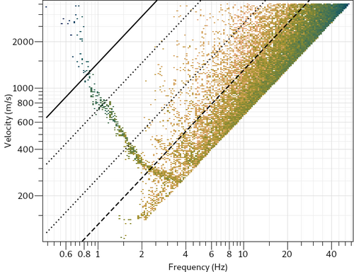
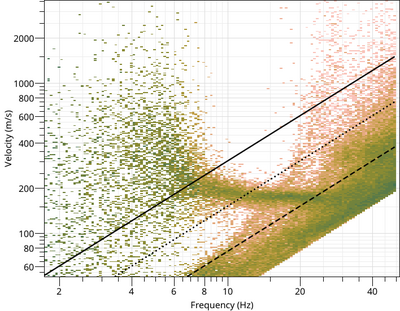
The input parameters are automatically adjusted and results are saved in file 'capon-C_135_405-Z.max'. By default,

• the minimum velocity is set to 50 m/s,
• time windows are 50-period long,
• the cross-spectrum matrix is calculated by averaging 2N blocks (time windows) where N is the the number of sensors,
• the minimum frequency is set to have at least two velocity estimations (taking block average parameters and gaps into account),
• the maximum frequency is set to Nyquist frequency,
• the number of peaks searched on the FK map is limited to N with a minimum relative threshold of 90% for their amplitude (the reference is the highest peak).

Dispersion curve obtained with the vertical component high resolution FK (manual limits).

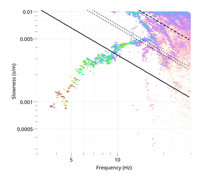
The results can be viewed with:

 $ gpviewmax capon-C_135_405-Z.max

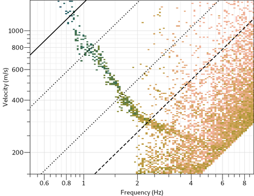
The high frequency limit based on Nyquist frequency is far too high for this array. The aliasing limit deduced from Kmax (Wathelet et al., 2008) is too restrictive. A curve can certainly be delineated above 4 Hz. Processing parameters can be adjusted in a file:

 $ geopsy-fk -db Mirandola.gpy -group C_135_405-Z -param limits.param -o limited

where limits.param can be for instance:

 GRID_SIZE_FACTOR=4
 MAXIMUM_FREQUENCY=10
 MIN_V=150

Dispersion curve obtained with the vertical component high resolution FK (manual limits and maximum overlap at 100%).

Dispersion curve obtained with the vertical component high resolution FK (manual limits and maximum overlap at 100%).

Option -o adds a prefix to the automatic output file name which is by default process_type-group_name.max. Parameters can be also modified directly in the command line:

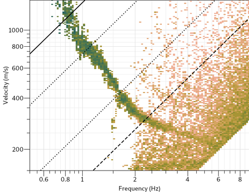
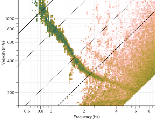
 $ geopsy-fk -db Mirandola.gpy -group C_135_405-Z -param limits.param -o limited -set STATISTIC_MAX_OVERLAP=100 -set STATISTIC_COUNT=0

The parameters are first loaded from limits.param, then STATISTIC_MAX_OVERLAP is set to 100% instead of 0% and STATISTIC_COUNT is set to 0 instead of 50. The order of the options -param and -set matters and they can be used several times. At 100% overlap, successive block sets re-use the same same blocks, sliding by the minimum increment, that is, just one block. The number of phase velocity samples per frequency band is controlled by STATISTIC_COUNT. According to length of blocks and the number of required samples, the block set increment might be larger than the minimum of one. A null STATISTIC_COUNT removes the limitation of the number of samples (time consuming, particularly at high frequency).

There are many other secondary parameters. To get a list of all possible parameters and their default values, run:

 $ geopsy-fk -param-example

.max files save the command line arguments, the version of geopsy-fk and its dependencies, the parameters and the results. The history of arguments can be also accessed through

 $ geopsy-fk -args

geopsy-fk and gpviewmax support help option.

 $ geopsy-fk -h all

The next table provides a rough idea of the time spent for various configurations. These estimations were all made on an Intel(R) Core(TM) i7-8650U at 1.9 GHz (cache: L1=32 KB, L2=256 KB, L3=8192 KB). There are 4 physical cores (+4 with hyper-threading).

Parameters	Platform	Threads	CPU time
Default	Debian 11	4	54 sec.
Default, direct file access	Debian 11	4	1 min. 18 sec.
Default	Debian 11	8	sec.
limits.param	Debian 11	4	43 sec.
limits.param, STATISTIC_MAX_OVERLAP=100	Debian 11	4	2 min. 8 sec.
limits.param, STATISTIC_MAX_OVERLAP=100, STATISTIC_COUNT=0	Debian 11	4	22 min. 5 sec.

Single component conventional FK

Dispersion curve for the conventional FK processed on the vertical component.

To run a conventional FK without block averaging as in geopsy graphical user interface before 2018:

 $ geopsy-fk -db Lep_ring01_3C.gpy -group vertical -set PROCESS_TYPE=Conventional -set BLOCK_COUNT=1 -set STATISTIC_COUNT=0

All-component Rayleigh ellipticity Direct Steering (ARDS)

File:Lep dc rayleigh ards.png

Dispersion curve for Rayleigh with ARDS.

The method is described in Wathelet (2024) .

 $ geopsy-fk -db Lep_ring01_3C.gpy -group 3C

The phase velocity, the ellipticity, the noise parameters, the azimuth and the beam power are view with

 $ gpviewmax ards-3C.max

Rayleigh Three-component BeamForming (RTBF)

Dispersion curve for Rayleigh with RTBF.

Ellipticity curve for Rayleigh with RTBF.

Estimation of the ratio of incoherent over coherent noise with RTBF.

Dispersion curve for Love with RTBF.

The method is described in Wathelet et al. (2018) . A typical parameter file can be (e.g. rtbf.param):

 MINIMUM_FREQUENCY=1
 MAXIMUM_FREQUENCY=30
 FREQ_BAND_WIDTH=0.1
 PROCESS_TYPE=RTBF
 ROTATE_STEP_COUNT=72
 BLOCK_COUNT_FACTOR=4
 MIN_V (m/s)=100
 STATISTIC_MAX_OVERLAP(%)=100
 RELATIVE_THRESHOLD (%)=10

Parameter STATISTIC_MAX_OVERLAP adjusts the overlap between two block sets. At 100%, the block set is shifted by one block. At 0%, the block set is shifted by the number of blocks in the block set to avoid any overlap. Any intermediate value is possible. To run a three-component FK:

 $ geopsy-fk -db Lep_ring01_3C.gpy -group-path 3C -param rtbf.param

Note that the selected group must have the three components available for all sensors.

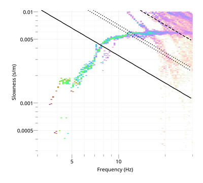
To view the Rayleigh dispersion curve:

 $ gphistogram rtbf-3C.max -p R

The option -p defines a pattern to select the result lines of file .max which contains a polarization column either Vertical, Rayleigh or Love. To view the Love dispersion curve:

 $ gphistogram rtbf-3C.max -p L

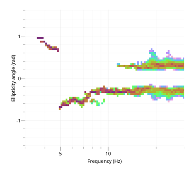
Love dispersion curve is computed in the same way as in Poggi et al. (2010) . To view the Rayleigh ellipticity curve:

 $ gphistogram rtbf-3C.max -p R -ell-angle

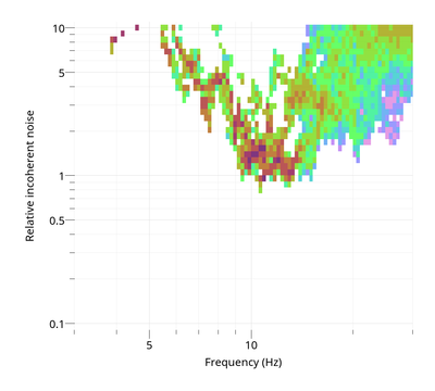
To view the ratio of incoherent over coherent noise:

 $ gphistogram rtbf-3C.max -p R -noise

Miscellaneous

The produced .max files contain an application signature in the header. The signature lists the arguments and the code version (with the Git commit ID). To re-run a case, for instance with new options or a new version, the .max file can be directly executed in a shell (from geopsypack-3.4.2).

 bash old_results-rtbf-group1.max

New options can be added.

  bash old_results-rtbf-group1.max -o new_results

The last option avoids overwriting the original file "old_results-rtbf-group1.max". Even if the original arguments had an option "-o", only the last one is kept.

References

- ↑ Garofalo, F., Foti, S., Hollender, F., Bard, P., Cornou, C., Cox, B. R., Ohrnberger, M., Sicilia, D., Asten, M., Di Giulio, G., Forbriger, T., Guillier, B., Hayashi, K., Martin, A., Matsushima, S., Mercerat, D., Poggi, V., Yamanaka, H. (2016). InterPACIFIC project: comparison of invasive and non-invasive methods for seismic site characterization. Part I: intra-comparison of surface wave methods, Soil Dynamics and Earthquake Engineering, 82, 222-240, 10.1016/j.soildyn.2015.12.010
- ↑ Wathelet, M., D. Jongmans, M. Ohrnberger, and S. Bonnefoy-Claudet (2008). Array performances for ambient vibrations on a shallow structure and consequences over Vs inversion. Journal of Seismology, 12, 1-19. , 10.1007/s10950-007-9067-x
- ↑ Marc Wathelet, Incoherent noise-induced distortions of Rayleigh wave ellipticity measurements obtained with three-component beamforming, Geophysical Journal International, 2024, 10.1093/gji/ggae017
- ↑ Wathelet, M, Guillier, B, Roux, P, Cornou, C. and Ohrnberger, M., Rayleigh wave three-component beamforming: signed ellipticity assessment from high-resolution frequency-wavenumber processing of ambient vibration arrays, Geophysical Journal International, 215(1), 507-523, 10.1093/gji/ggy286
- ↑ Poggi, V. and Fäh, D., 2010, Estimating Rayleigh wave particle motion from three-component array analysis of ambient vibrations, Geophysical Journal International, 180(1), 251–267