Gplivemodel: Dispersion curve tutorial
First steps
- Start gplivemodel
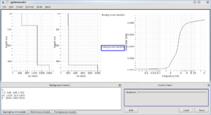
- Set this model as the background model:
3
7.5  500  200 1700
25  1350  210 1900
0   2000 1000 2500
- Set the same model as the reference model
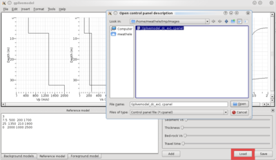
- Load control sliders from this setup. By creating new sliders, the foreground model is generated from reference model (see Foreground model tab in bottom left pane). Two profiles are visible on the plots.
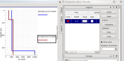
- Clearly identify background and foreground models by setting different colors for background and foreground models. Double click on legends located on the left of the dispersion curve plot. In the legend properties, set at least one entry for each legend. Adjust colors and other attributes to your taste.
- Play with slider controls. You may eventually freeze axis limits by unchecking option Automatic limits in menu Format. Set Sediment Vs and Travel time to their minimum value, and Thickness and Bed-rock Vs to their maximum before freezing limits. This way you get the largest ranges for axis values.
Slider definition
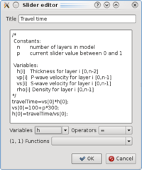
This section details the content of the slider control setup loaded in the previous section. Right click on any of them and select Edit to view or edit the attached code.
- Sediment Vs
vs[0]=100+p*400;
- Thickness
h[0]=5+p*50;
- Bed-rock Vs
vs[2]=250+p*1000;
- Travel time
travelTime=vs[0]*h[0];
vs[0]=100+p*300;
h[0]=travelTime/vs[0];
Click on Add button to create your own slider. Save button lets you save the current list of slider controls as a '.cpanel' file.
Type of curve
By default the fundamental mode of Rayleigh wave is computed. To switch to higher modes or Love modes, command line options at gplivemodel startup must be added (from a terminal, a MS-DOS console or a MSYS terminal)
- Fundamental Love mode only
gplivemodel -L 1 -R 0
- Rayleigh fundamental and first higher mode
gplivemodel -R 2
- Love fundamental and first higher mode
gplivemodel -R 0 -L 2
- Rayleigh fundamental group velocity
gplivemodel -R 1 -group


