Difference between revisions of "Geopsy: H/V and Spectrum Toolboxes: Output Tab"
| (42 intermediate revisions by 4 users not shown) | |||
| Line 1: | Line 1: | ||
| + | == Use == | ||
[[Image:HV_SPEC_toolb_output.png|thumb|right|300px|''Output'' tab where the user can fix the parameters to display and save the results]] | [[Image:HV_SPEC_toolb_output.png|thumb|right|300px|''Output'' tab where the user can fix the parameters to display and save the results]] | ||
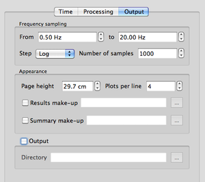
Through this tab, the user is able to fix the parameters to display and save the results. | Through this tab, the user is able to fix the parameters to display and save the results. | ||
| − | This tab is divided in three sections | + | This tab is divided in three sections: |
| − | * ''Frequency sampling'' section: where the user can fix the parameters on frequency limits and more | + | * ''Frequency sampling'' section: where the user can fix the parameters on frequency limits and more. |
| − | * ''Appearance | + | * ''Appearance'' section: where the user can fix automatic output graphics appearance parameters. |
| − | * ''Output | + | * ''Output'' section: where the user can fix where to save data. |
| + | <br style="clear: both"/> | ||
| + | == Frequency sampling section == | ||
| − | + | [[Image:HV_SPEC_toolb_output_frequency.png|thumb|left|300px|''Frequency sampling'' section used to define the parameters for frequency computing and displaying ]] | |
| + | |||
| + | <br style="clear: both"/> | ||
| + | Used to define the frequency processing and displaying parameters: | ||
| − | + | * The frequency lower (From) and upper (to) bounds of the frequency range of interest. | |
| − | + | The maximum upper bound frequency is determined by the [[Wikipedia:Nyquist_frequency|Nyquist frequency]], which corresponds to the half of the frequency data recording sampling (sps), above which no data are available. | |
| + | If the T10 limit has been checked in the [[Geopsy: Preferences#Tool plugins preferences|''Preferences'']], the reliable frequency range for the computation. Frequencies lower than the minimum reliable frequency are hatched in red. The minimum reliable frequency Fmin is estimated from the window length : Fmin= 10/(window length) | ||
| − | * | + | * Step: define how the sampling of the [[Geopsy:_Fast_Fourier_Transform|Fourier transform]] will be distributed. Two possibilities are available: |
| − | + | Lin: the samples are linearly distributed. | |
| − | |||
| + | Log: the samples are logarithmically distributed. | ||
| + | * Number of samples: number of samples used to process the [[Geopsy:_Fast_Fourier_Transform|Fourier transform]]. | ||
| − | |||
| − | |||
== Appearance section == | == Appearance section == | ||
| + | It is possible to customize the output graphics appearance, which may then be automatically applied on both single and summary output graphics. | ||
| + | |||
| + | |||
| + | [[Image:HV_SPEC_toolb_output_appearance.png||thumb|left|300px|''Appearance'' section.]] | ||
| + | |||
| + | First check the ''Results make-up'' and/or the ''Summary make-up'' box. Then open the browser by clicking on the neighborhing cursor [[Image:SPEC_cursor.png]] and choose the appropriate [[SciFigs: Make-up|make-up]] to apply to the output graphics so as to change its appearance. | ||
| + | |||
| + | When processing several files at the same time, single graphics output are displayed on the same page. The number of individual graphics to be displayed per line may be determined with the ''Plots per line'' spin box, and the page heigth adjusted with the ''Page heigth'' spin box. | ||
| + | <br style="clear: both"/> | ||
| − | |||
== Output section == | == Output section == | ||
| − | where to save data [[Image: | + | [[Image:HV_SPEC_toolb_output_output.png||thumb|right|300px|Unactivated ''Output'' section. Data is not saved.]][[Image:HV_SPEC_toolb_output_output_activated.png||thumb|right|300px|Activated ''Output'' section displaying in wich directory data will be saved.]] |
| + | [[Image:HV_SPEC_toolb_output_output_browser.png||thumb|right|300px|Browser to choose the folder to save the results. It is possible to create a new folder.]] | ||
| + | |||
| + | Results and processing parameters can be saved automatically while processing or after viewing the results. First check the ''Output'' box. Then open the file browser by clicking on the ''browse'' button [[Image:SPEC_cursor.png]] and select the folder where to save the output files. | ||
| + | |||
| + | <u>Note</u>: the output box must be checked and the destination folder selected '''before''' processing data, otherwise output files are not created. | ||
| + | |||
| + | |||
| + | The H/V and Spectrum output files are different: | ||
| + | |||
| + | * H/V processing<br/>For each H/V curve two output files are created: a parameter file, ''name.log'', and a result file, ''name.hv'', where "''name''" stands for the station name. | ||
| + | ** the ''.log'' file contains the H/V processing parameters and the windowing ([[Geopsy: H/V_parameter_file|Example]]). | ||
| + | ** the ''.hv'' file contains the H/V curve ([[Geopsy: H/V_output_file|Example]]). | ||
| + | |||
| + | |||
| + | * Spectrum processing<br/>For each component (Z, N, and E) two output files are created: a parameter file, ''name_component.log'', and a result file, ''name_component.spec'', where "name" stands for the station name. | ||
| + | ** the ''.log'' files contain the Spectrum processing parameters and the windowing ([[Geopsy: Spectrum_parameter_file|Example]]). | ||
| + | ** the ''.spec'' files contains the Fourier spectra curves ([[Geopsy: Spectrum_output_file|Example]]). | ||
| + | <br style="clear: both"/> | ||
| + | |||
| + | If the output files already exist, a pop-up warning window is displayed. | ||
| + | |||
| + | [[Image: File .log already exists HV.png||thumb|left|300px|H/V pop-up warning window]] | ||
| + | |||
| + | [[Image: File .log already exists Spec.png||thumb|left|400px|Spectrum pop-up warning window]] | ||
| − | = | + | <br style="clear: both"/> |
| − | |||
Latest revision as of 12:32, 10 January 2013
Use
Through this tab, the user is able to fix the parameters to display and save the results.
This tab is divided in three sections:
- Frequency sampling section: where the user can fix the parameters on frequency limits and more.
- Appearance section: where the user can fix automatic output graphics appearance parameters.
- Output section: where the user can fix where to save data.
Frequency sampling section
Used to define the frequency processing and displaying parameters:
- The frequency lower (From) and upper (to) bounds of the frequency range of interest.
The maximum upper bound frequency is determined by the Nyquist frequency, which corresponds to the half of the frequency data recording sampling (sps), above which no data are available. If the T10 limit has been checked in the Preferences, the reliable frequency range for the computation. Frequencies lower than the minimum reliable frequency are hatched in red. The minimum reliable frequency Fmin is estimated from the window length : Fmin= 10/(window length)
- Step: define how the sampling of the Fourier transform will be distributed. Two possibilities are available:
Lin: the samples are linearly distributed.
Log: the samples are logarithmically distributed.
- Number of samples: number of samples used to process the Fourier transform.
Appearance section
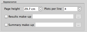
It is possible to customize the output graphics appearance, which may then be automatically applied on both single and summary output graphics.
First check the Results make-up and/or the Summary make-up box. Then open the browser by clicking on the neighborhing cursor ![]() and choose the appropriate make-up to apply to the output graphics so as to change its appearance.
and choose the appropriate make-up to apply to the output graphics so as to change its appearance.
When processing several files at the same time, single graphics output are displayed on the same page. The number of individual graphics to be displayed per line may be determined with the Plots per line spin box, and the page heigth adjusted with the Page heigth spin box.
Output section
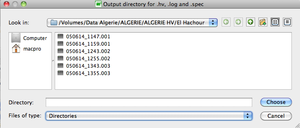
Results and processing parameters can be saved automatically while processing or after viewing the results. First check the Output box. Then open the file browser by clicking on the browse button ![]() and select the folder where to save the output files.
and select the folder where to save the output files.
Note: the output box must be checked and the destination folder selected before processing data, otherwise output files are not created.
The H/V and Spectrum output files are different:
- H/V processing
For each H/V curve two output files are created: a parameter file, name.log, and a result file, name.hv, where "name" stands for the station name.
- Spectrum processing
For each component (Z, N, and E) two output files are created: a parameter file, name_component.log, and a result file, name_component.spec, where "name" stands for the station name.
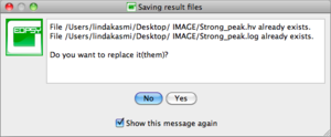
If the output files already exist, a pop-up warning window is displayed.


