Difference between revisions of "Ambient vibration array"
| Line 181: | Line 181: | ||
The basic idea of f-k processing consists of delaying the observed recordings at different stations according | The basic idea of f-k processing consists of delaying the observed recordings at different stations according | ||
| − | to a particular horizontal wavenumber vector <math>\vec{k}=(k_x,k_y)^T</math> and computing the coherence and/or beam power of the | + | to a particular horizontal wavenumber vector <math>\vec{k}=(k_x,k_y)^T</math> and computing the semblance coefficient <math>Semb(\omega,\vec{k})</math> (coherence measure) and/or beam power |
| − | shifted stacked output of all array stations. | + | <math>BP(\omega,\vec{k})</math> of the shifted stacked output of all array stations. |
| + | Beampower and Semblance are defined as follows: | ||
* Beampower: | * Beampower: | ||
| Line 194: | Line 195: | ||
</math> | </math> | ||
| − | <math>X_i(\omega)</math> is the observed record at station <math>i</math> at frequency <math>\omega</math>. The station coordinates | + | In the above formulas <math>X_i(\omega)</math> is the observed record at station <math>i</math> at frequency <math>\omega</math>. The station coordinates in the array plane (usually earth's surface) |
| − | in the array plane (usually earth's surface) are given by <math>\vec{r}_i</math>. | + | are given by <math>\vec{r}_i</math>. Therefore, the time delays of a harmonic plane wave |
| − | By testing many wavenumber vectors in the wavenumber plane one tries to find those | + | propagating along the horizontal plane in direction of <math>\vec{k}</math> and apparent propagation |
| − | array output. The wavenumber found corresponds to a plane wave along the surface crossing the seismometer array | + | velocity <math>c</math> related to the absolute length of the wavenumber vector <math>\|\vec{k}\| = 2\pi/\lambda = 2\pi f/c = \omega/c</math> can be computed as <math>\tau = \vec{k}\vec{r}_i</math>. |
| − | + | Thus, the beampower/semblance measure the power/coherence of a plane wave propagating with wavenumber | |
| − | + | vector <math>\vec{k}</math>. | |
| + | By testing many wavenumber vectors in the wavenumber plane one tries to find those wavenumber | ||
| + | vectors which maximize the array output. The wavenumber found corresponds to a plane wave | ||
| + | along the surface crossing the seismometer array. | ||
| + | So, the problem at hand is a general optimization problem trying to find the maximum | ||
| + | of a function of two parameters (here <math>(k_x,k_y)^T</math>). In order to optimize | ||
| + | the grid search approach, the f-k toolbox relies on an iterative refined sampling strategy. | ||
| + | In the first iteration potential maxima are identified within the search limits of the | ||
| + | wavenumber plane using a ''coarse'' grid step in both axis directions <math>(k_x,k_y)</math>. | ||
| + | Note, that ''coarse'' is relative and must be fine enough in order to match the goal: identifying | ||
| + | potential maxima in the wavenumber plane. Therefore, the grid step must be as small enough as to | ||
| + | sample the peaky structure of the [[Wikipedia:Array Response|array reponse]] sufficiently fine | ||
| + | for not missing any small maximum in the optimization procedure. The [[Wikipedia:Array Response|array response]] is closely related to the 2-dimensional [[Wikipedia:Array geometry|array geometry]]. In particular | ||
| + | the width of the main lobe peak - we refer to it as <math>k_{min}</math> - in the array response | ||
| + | (which is the one we are looking for) is approximately related to the overall aperture of the | ||
| + | array <math>D_{max}</math> by <math>k_{min} \approx 2\pi / D_{max}</math>. | ||
| + | |||
| + | In the current version of the f-k toolbox, the grid_step for sampling is automatically calculated as | ||
| + | <math>grid\_step = k_{min}/4</math>. Thus, any potential peak to be indentified in the wavenumber | ||
| + | domain will be sampled in either direction at least with four samples. | ||
<br style="clear: both"/> | <br style="clear: both"/> | ||
Revision as of 07:52, 9 March 2010
Contents
- 1 Common pre-requisites for array processing - getting ready
- 2 F-K Toolbox (conventional f-k)
- 3 High resolution frequency wavenumber Toolbox (Capon's method)
- 4 Modified Spatial Autocorrelation (MSPAC) Toolbox
Common pre-requisites for array processing - getting ready
Loading signals
View time series
Group signals
Insert / edit station coordinates
F-K Toolbox (conventional f-k)
Opening f-k toolbox - overview
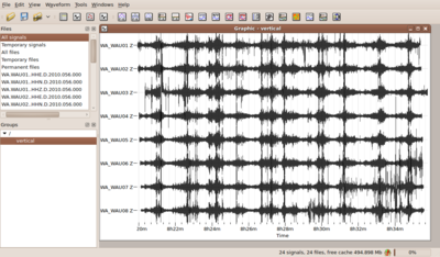
If you have followed all steps above you should have now a set of simultaneously recorded waveforms building a group and containing coordinates for each waveform. You can view this group of waveforms in the data viewer and should get a picture like the one shown to the right.
Now you can open the conventional frequency wavenumber toolbox by pushing the plugin icon ![]() .
.
The f-k toolbox should open and is now attached to the signal viewer. No other toolbox will now open with the signals you have loaded to the signal viewer. In order to process the same data set by another tool, you have to open them in a different signal viewer window. Note also, that once you close either the f-k toolbox window or the signal viewer, there is no way to undo this action - you will have to start again by opening a new signal viewer and attaching the f-k toolbox to it. Alternatively you can drag your group directly into the f-k toolbox icon. Geopsy will automatically open a new exclusively attached signal viewer for you.
Let's now have a close look to the individual parameters to be set in the f-k toolbox. There are four main groups of parameters to be considered.
- Pre-processing parameters for excluding data from processing.
- Processing parameters for selecting time windows on the remaining data.
- Processing parameters for selecting narrow frequency bands for processing
- Parameters related to the output of results from f-k processing.
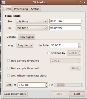
These parameters are laid out in different parts of the f-k toolbox widget. Note, that the toolbox has three main tabs: Time, Processing and Status.
The pre-processing parameters for excluding data from processing follow the same argumentation as the data selection for other toolboxes like H/V processing and can be found in the Time tab.
E.g. one can apply the so-called anti-trigger approach for removing transient signals from the continuous recordings (i.e. excluding those time chunks from processing). The anti-trigger approach can be applied to raw or filtered data. For the detailed settings please look into the description of anti-trigger. Another, second, approach for excluding data from processing is provided via the bad sample approach. For details in setting parameters with the bad sample approach check this page.
Parameter settings
Parameters for time window settings
There are two distinct inputs in the f-k toolbox for selecting time windows for processing. First, it is necessary to specify start and end times of the overall data window for processing by selecting entries From and To in the Time limits part of the Time tab of the fk-toolbox.
There are three options each for the
drop boxes From and To. For the From entry you can select among 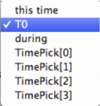 .
.
- this time (entries in form xx h xx m xx.xxx s)
- T0 (selects earliest common start time of all traces in group)
- during (selects time duration before end of the signals - either specified with End or this time as explained below)
For the To entry there are the options 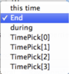 :
:
- this time (entries in form xx h xx m xx.xxx s)
- End (selects latest common end time of all traces in group)
- during (selects time duration from start time as given above - either specified by this time or T0)
Note: a selection of time limits as From: during && To: during is NOT valid.
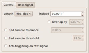
After selecting the overall data window for processing you finally have to specify the window length for
each single analysis window to be processed. You can find this Length parameter in the General tab inside the
Time tab. There are again three options provided in a drop box ![]() .
.
- Exactly (takes exactly the time window length as provided in the corresponding editable box - unit is in seconds).
- At least (takes at least the time window length as given in the editable box, if possible it takes more - unit is in seconds).
- Freq. dep. (read: frequency dependent. Scales window length to the center frequency of each frequency band to be processed. The number given in the editable box corresponds to a window length in number of cycles for each frequency band. T is the center period of the band).
Note: the most common setting for the Length parameter is Freq. dep. with values between 20.00 to 50.00 meaning that 20 to 50 cycles of the central signal period per frequency bands are used as window length. Example: for a frequency band with center frequency 2.5 Hz, the central period is 1/2.5 = 0.4 s. Therefore, with a frequency dependent Length setting of 30.00 T, the window length will be chosen as 12.00 s.
Parameters for frequency band selection
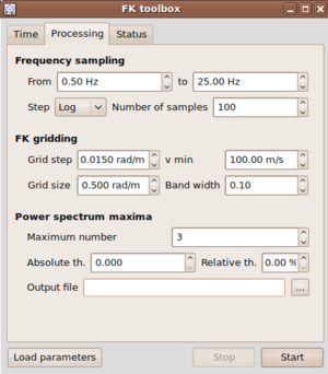
The selection of the frequency bands to be processed is driven by parameter inputs inside the Processing tab of the f-k toolbox.
In the Frequency sampling layout group you can specify the minimum and the maximum (central) frequencies for processing.
Between these two limits, the frequency axis will then be sampled according to the settings in the next line  .
.
There are two options to be specified, namely Step and Number of Samples. For the Step parameter, there are two options to be selected from a drop box: Log or Linear. You might have guessed the meaning right away. When choosing Linear then the frequency axis is sampled linearly between the given limits and exactly Number of Samples will be distributed along the axis. Choosing Log accordingly samples the frequency axis logarithmically, i.e. frequency bands are close spaced at lower frequencies.
Note: the sampled frequencies are taken as center frequencies in the processing scheme. Therefore, it is necessary to specify additionally a bandwidth
so that the processing can be performed in a finite but narrow frequency band. The bandwidth parameter is chosen as relative half-bandwidth in the FK-gridding layout group in the processing tab  .
.
The frequency limits for each frequency band are computed as Failed to parse (MathML with SVG or PNG fallback (recommended for modern browsers and accessibility tools): Invalid response ("Math extension cannot connect to Restbase.") from server "https://wikimedia.org/api/rest_v1/":): {\displaystyle [(1-bw)\cdot f_c,(1+bw)\cdot f_c] } where Failed to parse (MathML with SVG or PNG fallback (recommended for modern browsers and accessibility tools): Invalid response ("Math extension cannot connect to Restbase.") from server "https://wikimedia.org/api/rest_v1/":): {\displaystyle f_c} is the central frequency and Failed to parse (MathML with SVG or PNG fallback (recommended for modern browsers and accessibility tools): Invalid response ("Math extension cannot connect to Restbase.") from server "https://wikimedia.org/api/rest_v1/":): {\displaystyle bw} is the bandwidth parameter.
Example: a setting of 0.10 for the bandwidth, a Linear spacing of 10 samples along the frequency axis from 1 Hz to 10 Hz will create the following frequency bands:
| Freq. band index | Lower frequency limit | Center frequency | Upper frequency limit |
|---|---|---|---|
| 1 | 0.9 Hz | 1.0 Hz | 1.1 Hz |
| 2 | 1.8 Hz | 2.0 Hz | 2.2 Hz |
| 3 | 2.7 Hz | 3.0 Hz | 3.3 Hz |
| 4 | 3.6 Hz | 4.0 Hz | 4.4 Hz |
| 5 | 4.5 Hz | 5.0 Hz | 5.5 Hz |
| 6 | 5.4 Hz | 6.0 Hz | 6.6 Hz |
| 7 | 6.3 Hz | 7.0 Hz | 7.7 Hz |
| 8 | 7.2 Hz | 8.0 Hz | 8.8 Hz |
| 9 | 8.1 Hz | 9.0 Hz | 9.9 Hz |
| 10 | 9.0 Hz | 10.0 Hz | 11.0 Hz |
Parameters influencing the sampling of the wavenumber space
The basic idea of f-k processing consists of delaying the observed recordings at different stations according to a particular horizontal wavenumber vector Failed to parse (MathML with SVG or PNG fallback (recommended for modern browsers and accessibility tools): Invalid response ("Math extension cannot connect to Restbase.") from server "https://wikimedia.org/api/rest_v1/":): {\displaystyle \vec{k}=(k_x,k_y)^T} and computing the semblance coefficient Failed to parse (MathML with SVG or PNG fallback (recommended for modern browsers and accessibility tools): Invalid response ("Math extension cannot connect to Restbase.") from server "https://wikimedia.org/api/rest_v1/":): {\displaystyle Semb(\omega,\vec{k})} (coherence measure) and/or beam power Failed to parse (MathML with SVG or PNG fallback (recommended for modern browsers and accessibility tools): Invalid response ("Math extension cannot connect to Restbase.") from server "https://wikimedia.org/api/rest_v1/":): {\displaystyle BP(\omega,\vec{k})} of the shifted stacked output of all array stations. Beampower and Semblance are defined as follows:
- Beampower:
Failed to parse (MathML with SVG or PNG fallback (recommended for modern browsers and accessibility tools): Invalid response ("Math extension cannot connect to Restbase.") from server "https://wikimedia.org/api/rest_v1/":): {\displaystyle BP(\omega,\vec{k}) = \sum_{\omega=\omega_l}^{\omega=\omega_h} \left[\sum_{i=1}^{i=N} X_i(\omega)\exp(j\vec{k}\vec{r}_i)\right]^2 }
- Semblance:
Failed to parse (MathML with SVG or PNG fallback (recommended for modern browsers and accessibility tools): Invalid response ("Math extension cannot connect to Restbase.") from server "https://wikimedia.org/api/rest_v1/":): {\displaystyle Semb(\omega,\vec{k}) = \frac{\sum_{\omega=\omega_l}^{\omega=\omega_h} \left[\sum_{i=1}^{i=N} X_i(\omega)\exp(j\vec{k}\vec{r}_i)\right]^2} {N \sum_{\omega=\omega_l}^{\omega=\omega_h}\sum_{i=1}^{i=N} \left[X_i(\omega)\exp(j\vec{k}\vec{r}_i)\right]^2} }
In the above formulas Failed to parse (MathML with SVG or PNG fallback (recommended for modern browsers and accessibility tools): Invalid response ("Math extension cannot connect to Restbase.") from server "https://wikimedia.org/api/rest_v1/":): {\displaystyle X_i(\omega)} is the observed record at station Failed to parse (MathML with SVG or PNG fallback (recommended for modern browsers and accessibility tools): Invalid response ("Math extension cannot connect to Restbase.") from server "https://wikimedia.org/api/rest_v1/":): {\displaystyle i} at frequency Failed to parse (MathML with SVG or PNG fallback (recommended for modern browsers and accessibility tools): Invalid response ("Math extension cannot connect to Restbase.") from server "https://wikimedia.org/api/rest_v1/":): {\displaystyle \omega} . The station coordinates in the array plane (usually earth's surface) are given by Failed to parse (MathML with SVG or PNG fallback (recommended for modern browsers and accessibility tools): Invalid response ("Math extension cannot connect to Restbase.") from server "https://wikimedia.org/api/rest_v1/":): {\displaystyle \vec{r}_i} . Therefore, the time delays of a harmonic plane wave propagating along the horizontal plane in direction of Failed to parse (MathML with SVG or PNG fallback (recommended for modern browsers and accessibility tools): Invalid response ("Math extension cannot connect to Restbase.") from server "https://wikimedia.org/api/rest_v1/":): {\displaystyle \vec{k}} and apparent propagation velocity Failed to parse (MathML with SVG or PNG fallback (recommended for modern browsers and accessibility tools): Invalid response ("Math extension cannot connect to Restbase.") from server "https://wikimedia.org/api/rest_v1/":): {\displaystyle c} related to the absolute length of the wavenumber vector Failed to parse (MathML with SVG or PNG fallback (recommended for modern browsers and accessibility tools): Invalid response ("Math extension cannot connect to Restbase.") from server "https://wikimedia.org/api/rest_v1/":): {\displaystyle \|\vec{k}\| = 2\pi/\lambda = 2\pi f/c = \omega/c} can be computed as Failed to parse (MathML with SVG or PNG fallback (recommended for modern browsers and accessibility tools): Invalid response ("Math extension cannot connect to Restbase.") from server "https://wikimedia.org/api/rest_v1/":): {\displaystyle \tau = \vec{k}\vec{r}_i} . Thus, the beampower/semblance measure the power/coherence of a plane wave propagating with wavenumber vector . By testing many wavenumber vectors in the wavenumber plane one tries to find those wavenumber vectors which maximize the array output. The wavenumber found corresponds to a plane wave along the surface crossing the seismometer array.
So, the problem at hand is a general optimization problem trying to find the maximum of a function of two parameters (here Failed to parse (MathML with SVG or PNG fallback (recommended for modern browsers and accessibility tools): Invalid response ("Math extension cannot connect to Restbase.") from server "https://wikimedia.org/api/rest_v1/":): {\displaystyle (k_x,k_y)^T} ). In order to optimize the grid search approach, the f-k toolbox relies on an iterative refined sampling strategy. In the first iteration potential maxima are identified within the search limits of the wavenumber plane using a coarse grid step in both axis directions Failed to parse (MathML with SVG or PNG fallback (recommended for modern browsers and accessibility tools): Invalid response ("Math extension cannot connect to Restbase.") from server "https://wikimedia.org/api/rest_v1/":): {\displaystyle (k_x,k_y)} . Note, that coarse is relative and must be fine enough in order to match the goal: identifying potential maxima in the wavenumber plane. Therefore, the grid step must be as small enough as to sample the peaky structure of the array reponse sufficiently fine for not missing any small maximum in the optimization procedure. The array response is closely related to the 2-dimensional array geometry. In particular the width of the main lobe peak - we refer to it as Failed to parse (MathML with SVG or PNG fallback (recommended for modern browsers and accessibility tools): Invalid response ("Math extension cannot connect to Restbase.") from server "https://wikimedia.org/api/rest_v1/":): {\displaystyle k_{min}} - in the array response (which is the one we are looking for) is approximately related to the overall aperture of the array Failed to parse (MathML with SVG or PNG fallback (recommended for modern browsers and accessibility tools): Invalid response ("Math extension cannot connect to Restbase.") from server "https://wikimedia.org/api/rest_v1/":): {\displaystyle D_{max}} by Failed to parse (MathML with SVG or PNG fallback (recommended for modern browsers and accessibility tools): Invalid response ("Math extension cannot connect to Restbase.") from server "https://wikimedia.org/api/rest_v1/":): {\displaystyle k_{min} \approx 2\pi / D_{max}} .
In the current version of the f-k toolbox, the grid_step for sampling is automatically calculated as Failed to parse (MathML with SVG or PNG fallback (recommended for modern browsers and accessibility tools): Invalid response ("Math extension cannot connect to Restbase.") from server "https://wikimedia.org/api/rest_v1/":): {\displaystyle grid\_step = k_{min}/4} . Thus, any potential peak to be indentified in the wavenumber domain will be sampled in either direction at least with four samples.
Saving results / contents of output file
There will be two output files created. The name of the output file and the location (path) for storing the output files is specified in the lowest layout group of the Processing tab titled Power spectrum maxima with the option Output file. Pushing the button to the right of the editable textbox entry will open a file browser and allows you to navigate to some location in your directory tree and specify an output file name.
The extension of the main output file is .max. Additionally an other output file is created containing the processing parameters and information created during
the processing run. The extension of this file is set to .log. Parameters can be reloaded from an existing .log file in the Load parameters option form the Time tab of the f-k toolbox ![]() .
.
# File generated by Geopsy, FK processing
# The process log is saved in file lep_ring01.log
# Header
# GRID_LAYOUT 0
# GRID_TYPE 0
# NPHI 72
# GRID_RESOL 250
# GRID_MAX 10
# NUM_BANDS 100
# Number of freq bands: 100
# Band 0 lower 0.45 center 0.5 upper 0.55
# Band 1 lower 0.468138 center 0.520153 upper 0.572169
# Band 2 lower 0.487007 center 0.541119 upper 0.595231
# Band 3 lower 0.506636 center 0.562929 upper 0.619222
# Band 4 lower 0.527057 center 0.585619 upper 0.644181
# Band 5 lower 0.548301 center 0.609223 upper 0.670146
# Band 6 lower 0.570401 center 0.633779 upper 0.697157
...............
...............
# Band 95 lower 19.2104 center 21.3449 upper 23.4794
# Band 96 lower 19.9847 center 22.2053 upper 24.4258
# Band 97 lower 20.7903 center 23.1003 upper 25.4103
# Band 98 lower 21.6282 center 24.0314 upper 26.4345
# Band 99 lower 22.5 center 25 upper 27.5
# seconds from start | cfreq | slow | az | math-phi | semblance | beampow
30378.9 0.940916 5.15376 21.9177 68.0823 0.491473 63.9522
30442.7 0.940916 3.18228 38.3304 51.6696 0.210185 65.6729
30474.6 0.940916 3.85247 121.714 328.286 0.298423 69.8839
30121.3 0.978841 4.66624 276.785 173.215 0.22663 70.1559
30366.6 0.978841 6.27949 18.5945 71.4055 0.188424 71.1481
30397.3 0.978841 6.79274 263.773 186.227 0.177627 63.9104
30354.7 1.0183 5.79576 65.0153 24.9847 0.192576 71.5275
30384.2 1.0183 6.28673 265.305 184.695 0.604842 71.942
30458.6 0.978841 4.57822 4.44118 85.5588 0.23338 69.5334
...........
...........
The contents of the output file are best explained by having a look into the plain ascii file. Header lines are marked with a # as the first character of the line. The header entries of the max files provide the list of frequency bands that were processed. Other entaa,ries are obsolete but are kept for compatibility with former file formats used in other codes during the SESAME project.
The more interesting lines of the the .max output file start right below the header lines. The final header line describes the entries in the different columns:
- Time from start of processed data window in seconds
- Center frequency of the processed data window
- Estimated Slowness in s/km (this unit is also kept for compatibility reasons)
- Azimuth of propagation direction (direction of wavenumber/slowness vector) as measured from North via East
- Same angle as before, but now given in mathematical orientation (measured from East via North)
- Semblance coefficient
- Beampower value given in dB ( Failed to parse (MathML with SVG or PNG fallback (recommended for modern browsers and accessibility tools): Invalid response ("Math extension cannot connect to Restbase.") from server "https://wikimedia.org/api/rest_v1/":): {\displaystyle 10\cdot \log(BP(\omega,\vec{k}))}
Log file - different sections
section init
### Init Log ###
*********** vertical ***********
Add signal id 3 to component Vertical of station WA_WAU01 at 0.940538 -0.0688223 43.6439
Add signal id 6 to component Vertical of station WA_WAU02 at 5.32643 4.2312 43.7266
Add signal id 9 to component Vertical of station WA_WAU03 at 5.72042 -4.39827 42.5163
Add signal id 12 to component Vertical of station WA_WAU04 at 0.230693 -8.01841 42.9798
Add signal id 15 to component Vertical of station WA_WAU05 at -2.61856 -4.15918 43.5125
Add signal id 18 to component Vertical of station WA_WAU06 at -6.41618 0.965644 43.5362
Add signal id 21 to component Vertical of station WA_WAU07 at -3.53215 4.06034 43.6112
Add signal id 24 to component Vertical of station WA_WAU08 at 0.34882 7.3875 43.6973
Found 8 different stations
### End Init Log ###
Parameter section - note this can be loaded via the Load Params button.
### Parameters ###
WINDOW MIN LENGTH (s) = 50
WINDOW MAX LENGTH (s) = 30
WINDOW LENGTH TYPE (at least/exactly/freq. dep.) = freq. dep.
DO BAD SAMPLE TOLERANCE (y/n) = n
BAD SAMPLE TOLERANCE (s) = 0
DO WINDOW OVERLAP (y/n) = n
WINDOW OVERLAP (%) = 5
DO BAD SAMPLE THRESHOLD (y/n) = n
BAD SAMPLE THRESHOLD (%) = 99
ANTI-TRIGGERING ON RAW SIGNAL (y/n) = n
USED RAW COMPONENTS = y, n, y, y, y, y, y, y, y, y
RAW STA (s) = 1
RAW LTA (s) = 30
RAW MIN SLTA = 0.2
RAW MAX SLTA = 2.5
MINIMUM FREQUENCY = 0.5
MAXIMUM FREQUENCY = 25
INVERSED FREQUENCY = n
SAMPLES NUMBER FREQUENCY = 100
SAMPLING TYPE FREQUENCY (0=log, 1=linear)= 0
FROM TIME TYPE = 0
FROM TIME TEXT = 8h21m0s
TO TIME TYPE = 0
TO TIME TEXT = 9h29m0s
MIN K = 0.015
MAX K = 0.5
MIN V = 100
FREQ BAND WIDTH = 0.1
N MAXIMA = 3
OUTPUT FILE = /home/mao/GEOPSY_DOC_WORKSHOP/lep_ring01.max
### End Parameters ###
Process Log section
### Process Log ###
Process started at 2010-03-08 10:54:47
Adding window from 30060 to 30120 s.
Adding window from 30120 to 30180 s.
Adding window from 30180 to 30240 s.
Adding window from 30240 to 30300 s.
Adding window from 30300 to 30360 s.
Adding window from 30360 to 30420 s.
Adding window from 30420.1 to 30480.1 s.
Adding window from 30480.1 to 30540.1 s.
Adding window from 30540.1 to 30600.1 s.
Adding window from 30600.1 to 30660.1 s.
Adding window from 30660.1 to 30720.1 s.
Adding window from 30720.1 to 30780.1 s.
Adding window from 30780.1 to 30840.1 s.
Adding window from 30840.1 to 30900.1 s.
Frequency 1/100 0.5
Min Window length 60 seconds
Max Window length 60 seconds
 14 Time windows
.......
Adding window from 30919.1 to 30920.3 s.
Adding window from 30920.3 to 30921.5 s.
Adding window from 30921.5 to 30922.7 s.
Frequency 100/100 25
Min Window length 1.2 seconds
Max Window length 1.2 seconds
 713 Time windows
Process run in 00:01:20
Process ended at 2010-03-08 10:56:08
### End Process Log ###
Graphical display of f-k results using max2curve
High resolution frequency wavenumber Toolbox (Capon's method)
The high resolution frequency wavenumber (hrfk) algorithm follows the ideas of Capon (1969) [1]
. The corresponding toolbox that can be called using the following
plugin icon ![]() can be used straightforward in nearly the same way
as the conventional f-k toolbox.
can be used straightforward in nearly the same way
as the conventional f-k toolbox.
There is just one more (optional!) parameter that can be set. The calcuation for the hrfk algorithm involves the inversion of the cross spectral matrix estimate from the data. In order to guarantee a numerically stable solution for the Matrix inversion, a regularization parameter (damping constant) can be provided to load the diagonal of the cross spectral matrix before inversion.
Note: by doing so (using a damping constant), you will smooth out your wavenumber power spectra and eventually not obtain much better results compared to the conventional beamforming approach.
Saving results / contents of output file
Graphical display of f-k results using max2curve
Modified Spatial Autocorrelation (MSPAC) Toolbox
The Modified Spatial Autocorrelation (MSPAC) was introduced by Bettig et al. (2001) [2] after pioneer paper of Aki (1957)[3]. This method allows computing spatial autocorrelation coefficients for any arbitary array layouts.
After viewing the group of waveforms in the data viewer, open the MSPAC toolbox by pushing the following plugin icon ![]() . Alternatively you can drag your group directly into the SPAC toolbox icon. The SPAC toolbox should now be attached to the signal viewer.
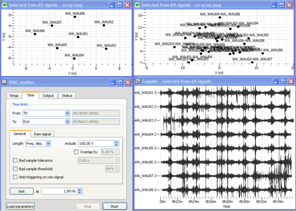
Four windows should then opened as displayed in the figure on the right: (1) a signal time viewer, (2) a map displaying array station locations, (3) a map displaying co-array stations location and (4) the SPAC processing toolbox. This processing toolbox is composed of four sub-menus: "Rings" sub-menu is used to design rings from the co-array; "Time" is used to define begin and end time to be processed, time window length, anti-triggering options as described in section XXX; "Output" menu is used to set up the output frequency band together with the sampling scale type (linear, log) and number of frequencies, the output filename; "Status" menu provides information about computing status. All these sub-menus are described hereafter.
. Alternatively you can drag your group directly into the SPAC toolbox icon. The SPAC toolbox should now be attached to the signal viewer.
Four windows should then opened as displayed in the figure on the right: (1) a signal time viewer, (2) a map displaying array station locations, (3) a map displaying co-array stations location and (4) the SPAC processing toolbox. This processing toolbox is composed of four sub-menus: "Rings" sub-menu is used to design rings from the co-array; "Time" is used to define begin and end time to be processed, time window length, anti-triggering options as described in section XXX; "Output" menu is used to set up the output frequency band together with the sampling scale type (linear, log) and number of frequencies, the output filename; "Status" menu provides information about computing status. All these sub-menus are described hereafter.
Defining rings
In "rings" sub-menu:
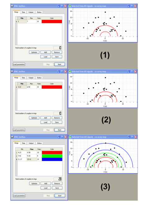
- Push on
 button to add a ring
 - Specify the inner and outer circles radii of the ring (see step (1) in the figure on the left)
- Press on
 buttom to adjust the inner and outer circles radii in order to fit at best sensors location (see step (2) in the figure on the left). This ring is composed of 10 pairs of sensors as specified in the "Pairs" column.
 - Define the next rings (see step (3) in the figure on the left). Note that you can associate a specific color to each ring.
- Note that you add or remove specific ring by pushing on the
 or
or  buttons
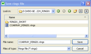
 - Once done, click on
 to save your rings design.
- The rings design can next be loaded by pushing on the
 button
 - the rings design are saved in ascii format with the following format: inner circle radius (in meters), outer circle radius (in meters), RGB color code associated to the ring
# MinRadius    MaxRadius   Red   Green  Blue
 4.23 ...
Defining time limits
In "Time" sub-menu:
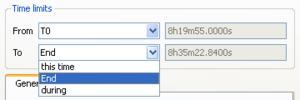
- Select the time limits to be processed. You can either use the begin To and end time End of the time series, either specify the begin and end time This Time or specify the time duration Duration
- Specify the window length that will be used for processing. You can either choose a window length that is inversely proportionnal to the frequency of interest Freq. Dep., a fixed time window length Exactly or a variable length limited by a minimum and a maximumm At Least.
- By pushing on
 , you can also load the .log file containing all the input parameters saved from a previous computation (see Editing spatial autocorrelation curves for complementary information).
Defining the outputs and starting the computation
In "Output" sub-menu:
- Choose the frequency band used for the computation
- Specify the number of frequencies and the sampling scale (constant on a linear or logarithmic scale).
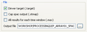
- Click on Dinver target to save your results in a .target file. Set the output filename.
- Then, click on
 to start the computation. Status of the computation can be checked in the "Status" sub-menu as displayed below.
Graphical display of spatial autocorrelation curves / contents of output files
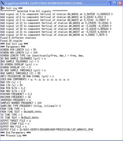
The spatial autocorrelation coefficients and the parameters used for the computation are saved in a .target binary file and a .log ascii file, respectively. The .log file is saved in the same folder as the .target file. The figure on the right displays the content of the .log file. The .target file is a binary file.
Graphical display of spatial autororrelation curves can be done by importing the .target file in the "target" menu of "Dinver" (CROSS-REFERENCE) or by using an utility called spac2disp that can be launched either from the windows Geopsy menu either from a command line
References
- ↑ Capon, 1969. xxx ,IEEE Proceedings, , , .
- ↑ Bettig B., P.-Y. Bard, F. Scherbaum, J. Riepl, F. Cotton, C. Cornou, D. Hatzfeld, 2001. Analysis of dense array measurements using the modified spatial auto-correlation method (SPAC). Application to Grenoble area., Boletin de Geofisica Teoria e Applicata, 42, 3-4, 281-304.
- ↑ Aki, K., 1957. Space and Time Spectra of Stationary Stochastic Waves, with Special Reference to Microtremors, Bull. Earthq. Res. Inst. Tokyo, 35, 415-457.
